Basic Equations
For the wave dynamics of the electric and magnetic fields in a dielectric waveguide, one seeks solutions of Maxwell’s equations with harmonic time dependence, so-called optical modes.
Maxwell’s equation in a dielectric medium are given by
$$
\begin{align}
\nabla \cdot \vec{D} &= \rho_f \tag{1.a} \\
\nabla \cdot \vec{B} &= 0 \tag{1.b} \\
\nabla \times \vec{E} &= - \partial_t \vec{B} \tag{1.c} \\
\nabla \times \vec{H} &= \vec{j}_f + \partial_t \vec{D} \tag{1.d}
\end{align}
$$
Only linear isotropic media are considered here, which yields constitutive relation:
$$
\begin{align}
\vec{D} &= \varepsilon_0 \varepsilon_r \vec{E} \tag{2.a} \\
\vec{B} &= \mu_0 \mu_r \vec{H} \tag{2.b}
\end{align}
$$
where $(\varepsilon_r) \varepsilon_0$ is the (relative) permittivity and $(\mu_r)\mu_0$ is the (relative) permeability.
They are related to refractive index $n=\sqrt{\varepsilon_r \mu_r}$ and vacuum speed of light $c= 1/\sqrt{\varepsilon_0 \mu_0}$
Furthermore it is assumed that no external currents and charges are present, $\vec{j}_f=0$ and $\rho_f=0$.
The boundary conditions at the interface between two isotropic materials with dielectric constants $\varepsilon_1$ and $\varepsilon_2$ are
$$
\begin{align}
\vec{\nu} \cdot (\varepsilon_1 \vec{E_1} - \varepsilon_2 \vec{E_2}) = 0 \tag{3.a} \\
\vec{\nu} \cdot (\vec{H_1} - \vec{H_2}) = 0 \tag{3.b} \\
\vec{\nu} \times (\vec{E_1} - \vec{E_2}) = 0 \tag{3.c} \\
\vec{\nu} \times (\vec{H_1} - \vec{H_2}) = 0 \tag{3.d}
\end{align}
$$
where $\varepsilon=\varepsilon_0 n^2$, assuming $\mu_r = 1$, which is typically the case.
Derivation of Wave Equation
$$
\begin{align}
\nabla \times \nabla \times \vec{E} &= \nabla (\nabla \cdot \vec{E}) - \nabla^2 \vec{E} = -\nabla^2 \vec{E} \tag{4.a} \\
\nabla \times \nabla \times \vec{H} &= \nabla (\nabla \cdot \vec{B})/\mu_0 - \nabla^2 \vec{H} = -\nabla^2 \vec{H} \tag{4.b}
\end{align}
$$
On the other hand,
$$
\begin{align}
\nabla \times \nabla \times \vec{E} &= \nabla \times (-\partial_t \vec{B}) = -\mu_0 \partial_t (\nabla \times \vec{H}) = -\mu_0 \partial^2_t \vec{D} = - \frac{n^2}{c^2} \partial^2_t \vec{E} \tag{5.a} \\
\nabla \times \nabla \times \vec{H} &= \nabla \times (\partial_t \vec{D}) = \varepsilon \partial_t (\nabla \times \vec{E}) = -\varepsilon \partial^2_t \vec{B} = - \frac{n^2}{c^2} \partial^2_t \vec{H} \tag{5.b}
\end{align}
$$
Eqs. (3.4a)-(3.5b) can be compactly written as the wave equation
$$
\begin{align}
\nabla^2 \vec{\Psi} \, (\vec{r},t) - \frac{n^2(\vec{r})}{c^2}\partial^2_t \vec{\Psi} \, (\vec{r},t) = 0 \tag{6}
\end{align}
$$
For $\vec{\Psi} \in$ {$\vec{E}, \vec{H}$}. A separation of variables leads to $\vec{\Psi}\,(\vec{r},t)=\vec{\Psi}\,(\vec{r}) exp(-i\omega t)$
The spatial distribution, the actual mode $\vec{\Psi}\,(\vec{r})$, is determined by the equaton
$$
\begin{align}
\nabla^2 \psi + n^2 k^2 \psi = 0 \tag{7}
\end{align}
$$
for every component $\psi$ of the field vector $\vec{\Psi}$
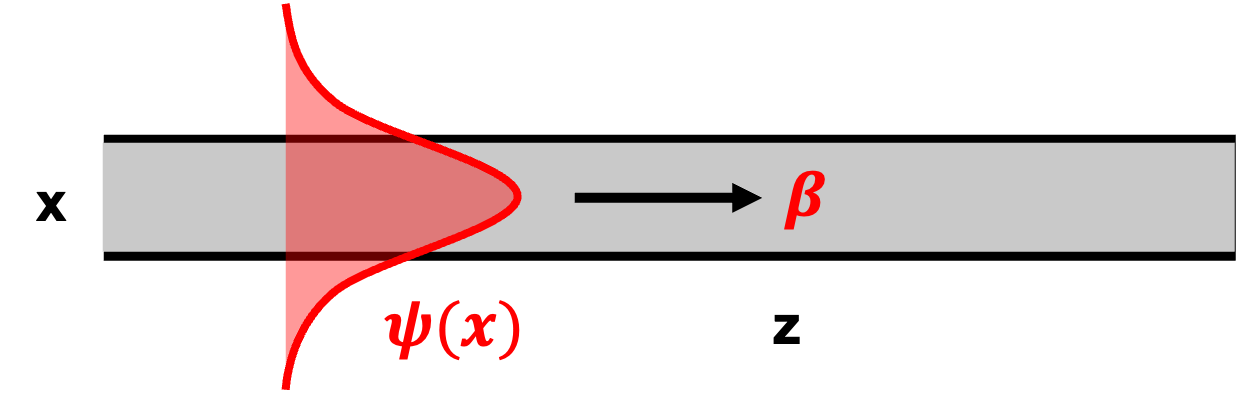
An eigenmode of waveguide structure is a propagating or evanscent wave of which the transversal shape does not change during propagation.
An eigenmode propagating in z-direction is represented by
$$
\begin{align*}
\vec{E} (\vec{r}) &= \vec{E}(x,y) e^{-i\beta z} \\
\vec{H} (\vec{r}) &= \vec{H}(x,y) e^{-i\beta z}
\end{align*}\tag{8}
$$
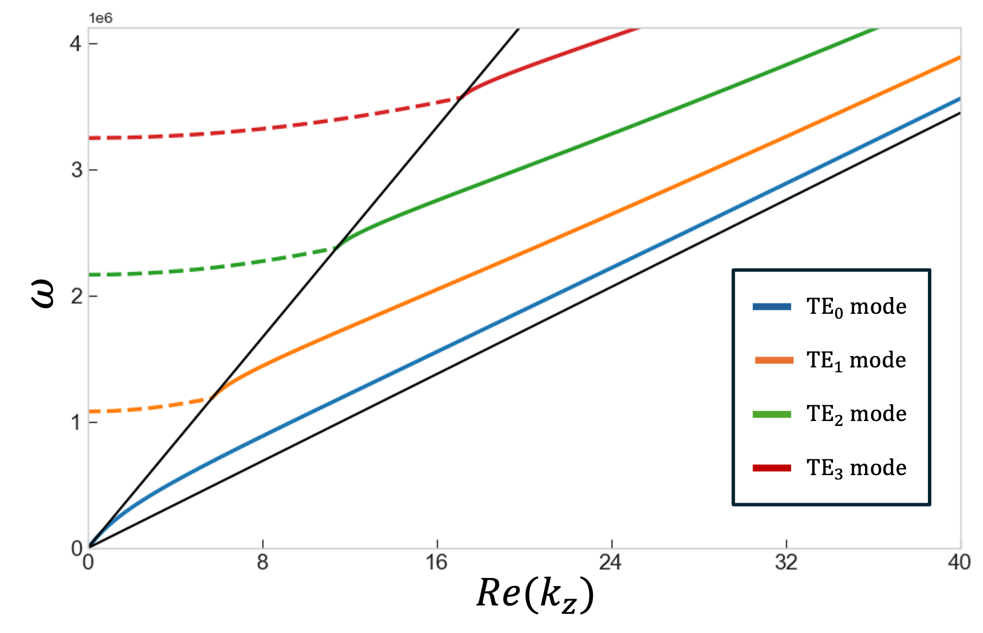
where $\beta$ is the propagation constant in the z-axis, which appears in the normalized form as $n_{\text{eff}} = \frac{\beta}{k}$.
Which makes equation (7)
$$
\begin{align}
\nabla^2 \psi (x,y) + (n^2(x,y) k^2 - \beta^2) \psi (x,y) = 0 \tag{9}
\end{align}
$$
Then the effective refractive index ($n_{eff} = \frac{\beta}{k}$) are in range
$$
\begin{align*}
n_{core} > n_{eff} > n_{clad} \quad (\text{for guided modes}) \\
\\
n_{clad} > n_{eff} \quad (\text{for radiative modes})
\end{align*}
$$
Guided modes and radiative modes form a complete set of functions.
$$
\begin{align*}
\vec{E}(x,y,z)=\sum_{m} a_m \vec{E}_m(x,y)e^{-i\beta_m z} + \int a(k) \vec{E}_k(x,y)e^{-ikz} \, dk \tag{10}
\end{align*}
$$
The Slab Waveguide
Consider Waveguides invariant in both the propagation and transverse directions
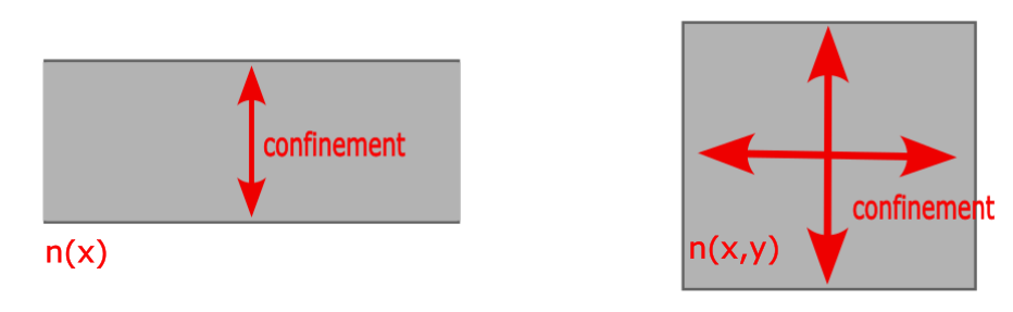
with $\vec{E} (\vec{r}) = \vec{E}(x) e^{-i\beta z}, \vec{H} (\vec{r}) = \vec{H}(x) e^{-i\beta z}$
Substituting these equations into Maxwell’s curl equations yields two independent electromagnetic modes: transverse electric (TE) and transverse magnetic (TM) polarizations.
$$
\begin{alignedat}{2}
\text{TE} \quad
&\left\{
\begin{aligned}
&\frac{d^2E_y}{dx^2} + (k^2n^2 - \beta^2)E_y = 0 \\
&H_x = - \frac{\beta}{\omega \mu_0}E_y \\
&H_z = - \frac{i}{\omega \mu_0} \frac{dE_y}{dx} \\
&E_x = E_z = H_y = 0
\end{aligned}
\right.
\qquad\qquad
&
\text{TM} \quad
&\left\{
\begin{aligned}
&\frac{d}{dx} \left( \frac{1}{n^2} \frac{dH_y}{dx} \right) + \left( k^2 - \frac{\beta^2}{n^2} \right) H_y = 0 \\
&E_x = \frac{\beta}{\omega \epsilon_0 n^2} H_y \\
&E_z = \frac{i}{\omega \epsilon_0 n^2} \frac{dH_y}{dx} \\
&H_x = H_z = E_y = 0
\end{aligned}
\right.
\end{alignedat}
$$
For these equations, we can derive the dispersion relations by applying the boundary conditions at the interfaces:
$$
\begin{aligned}
\left\{
\begin{aligned}
&E_{y,i}(a_i) = E_{y,i+1}(a_i) \\
&\frac{dE_{y,i}(a_i)}{dx} = \frac{dE_{y,i+1}(a_i)}{dx}
\end{aligned}
\right.
\end{aligned}
$$
to the general solution for each layer:
$$
\begin{aligned}
E_{y,i}(x) &= A_i e^{ik_{x,i}(x-a_i)} + B_i e^{-ik_{x,i}(x-a_i)} \\
\text{with}\quad
k_{x,i} &= \sqrt{k^2 n_i^2 - \beta^2}
\end{aligned}
$$
or to the ansatz for the TE mode:
$$
\begin{align*}
E_y(x) = \left\{
\begin{aligned}
&A \cos \left( k_x a - \phi \right) e^{-\sigma (x - a)}, \quad &x > a \\
&A \cos \left( k_x x - \phi \right), \quad &|x| \leq a \\
&A \cos \left( k_x a + \phi \right) e^{\gamma (x + a)}, \quad &x < -a
\end{aligned}
\right.
&&
\end{align*}
$$
where $k_x, \sigma, \gamma$ are wavenumbers along x-axis in each regions
then obtain the eigenvalue equations
$$
\begin{aligned}
k_x a &= \frac{m\pi}{2} + \frac{1}{2}\tan^{-1}(\frac{\gamma}{k_x}) + \frac{1}{2}\tan^{-1}(\frac{\sigma}{k_x}) \\
\phi &= \frac{m\pi}{2} + \frac{1}{2}\tan^{-1}(\frac{\gamma}{k_x}) - \frac{1}{2}\tan^{-1}(\frac{\sigma}{k_x})
\end{aligned}
$$
for the symmetrical waveguides with $n_0 = n_s$
$$
\begin{aligned}
k_x a &= \frac{m\pi}{2} + \tan^{-1}(\frac{\gamma}{k_x}) \\
\phi &= \frac{m\pi}{2}
\end{aligned}
$$